1. Introduction to the Qwen Model

In April 2023, Alibaba released the beta version of Qwen.

In December 2023, Alibaba open-sourced the first version of Qwen.

In September 2024, Alibaba released Qwen2.5.

In January 2025, Alibaba released Qwen 2.5-Max.

Qwen 2.5 is the latest series of the Qwen large language model. The reason it is called a series is that, after a pretrained model has been trained, we fine-tune, distill, prune, and quantize the model according to business scenarios and resource requirements to produce different models, so as to maximize the model’s value and strike a balance between performance and resource consumption for different purposes.

Besides the base model, Qwen2.5 also has versions fine-tuned for mathematics, programming, and instructions; parameter sizes range from 0.5 B to 72 B; there are also Int4 and Int8 quantized versions.

The Qwen series of large models has achieved excellent results on various leaderboards, and in our production environment some businesses also use models fine-tuned on the basis of Qwen.

2. Preparing the Environment

• Download Miniforge

1

wget "https://github.com/conda-forge/miniforge/releases/latest/download/Miniforge3-$(uname)-$(uname -m).sh"

• Install Miniforge

1

bash Miniforge3-$(uname)-$(uname -m).sh

• Configure variables

1
2

echo "export PATH=$HOME/miniforge3/bin:$PATH" >> ~/.bashrc
source ~/.bashrc

• Create an environment

1

conda create -n qwen python=3.12

• Activate the environment

1

conda activate qwen

• Download the model

1

git lfs clone https://huggingface.co/Qwen/Qwen2.5-0.5B

• Inspect the files

 1
 2
 3
 4
 5
 6
 7
 8
 9
10
11
12

tree Qwen2.5-0.5B

.
├── config.json
├── generation_config.json
├── LICENSE
├── merges.txt
├── model.safetensors
├── README.md
├── tokenizer_config.json
├── tokenizer.json
└── vocab.json

• Install dependencies

1

conda install transformers pytorch torchvision torchaudio pytorch-cuda=12.1 -c pytorch -c nvidia

3. Inspecting the Model Structure

• Specify the GPU number to use

1

export CUDA_VISIBLE_DEVICES=0

• Enter the IPython environment

1

conda install ipython

1

ipython

• Inspect the model structure

1
2
3
4

from transformers import AutoModelForCausalLM

model = AutoModelForCausalLM.from_pretrained("./Qwen2.5-0.5B")
print(model)

 1
 2
 3
 4
 5
 6
 7
 8
 9
10
11
12
13
14
15
16
17
18
19
20
21
22
23
24
25
26
27
28
29
30
31
32
33
34
35
36
37
38
39
40
41

Qwen2ForCausalLM(
# 这是一个 CausalLM 模型
  (model): Qwen2Model(
    (embed_tokens): Embedding(151936, 896)
    # 表示输入的词嵌入层，输入的词表大小为 151936，输出的维度为 896
    (layers): ModuleList(
      # 一共有 24 层 decoder 层
      (0-23): 24 x Qwen2DecoderLayer(
        # 自注意力层
        (self_attn): Qwen2Attention(
          # QKV 矩阵的维度, 输出维度为 896
          (q_proj): Linear(in_features=896, out_features=896, bias=True)
          (k_proj): Linear(in_features=896, out_features=128, bias=True)
          (v_proj): Linear(in_features=896, out_features=128, bias=True)
          (o_proj): Linear(in_features=896, out_features=896, bias=False)
        )
        # 前馈网络层，这里由 MLP 构成，
        (mlp): Qwen2MLP(
          # 门控线性层
          (gate_proj): Linear(in_features=896, out_features=4864, bias=False)
          # 上游投影
          (up_proj): Linear(in_features=896, out_features=4864, bias=False)
          # 下游投影
          (down_proj): Linear(in_features=4864, out_features=896, bias=False)
          # 激活函数shi
          (act_fn): SiLU()
        )
        # 多头注意力，输入特征维度为 896
        (input_layernorm): Qwen2RMSNorm((896,), eps=1e-06)
        # 对多头注意力输出特征进行归一化处理
        (post_attention_layernorm): Qwen2RMSNorm((896,), eps=1e-06)
      )
    )
    # 归一化处理，为下一层的输入做准备
    (norm): Qwen2RMSNorm((896,), eps=1e-06)
    # 位置编码，将位置信息加入到特征向量中
    (rotary_emb): Qwen2RotaryEmbedding()
  )
  # 线性层，将特征向量映射到词表大小
  (lm_head): Linear(in_features=896, out_features=151936, bias=False)
)

• Inspect the number of model parameters

1
2

num_params = sum(p.numel() for p in model.parameters())
print(f"模型参数总量: {num_params / 1e9:.5f} B")

1

模型参数总量: 0.49403 B

• Inspect the model configuration

1
2
3
4

from transformers import AutoConfig

config = AutoConfig.from_pretrained("./Qwen2.5-0.5B")
print(config)

 1
 2
 3
 4
 5
 6
 7
 8
 9
10
11
12
13
14
15
16
17
18
19
20
21
22
23
24
25
26
27
28
29
30

Qwen2Config {
  "_name_or_path": "./Qwen2.5-0.5B",
  "architectures": [
    "Qwen2ForCausalLM"
  ],
  "attention_dropout": 0.0,
  "bos_token_id": 151643,
  "eos_token_id": 151643,
  "hidden_act": "silu",
  "hidden_size": 896,
  "initializer_range": 0.02,
  "intermediate_size": 4864,
  "max_position_embeddings": 32768,
  "max_window_layers": 24,
  "model_type": "qwen2",
  "num_attention_heads": 14,
  "num_hidden_layers": 24,
  "num_key_value_heads": 2,
  "rms_norm_eps": 1e-06,
  "rope_scaling": null,
  "rope_theta": 1000000.0,
  "sliding_window": null,
  "tie_word_embeddings": true,
  "torch_dtype": "bfloat16",
  "transformers_version": "4.48.1",
  "use_cache": true,
  "use_mrope": false,
  "use_sliding_window": false,
  "vocab_size": 151936
}

Among them,

max_position_embeddings means the maximum sequence length supported by the model is 32768.

num_attention_heads is the number of heads in multi-head attention, and num_key_value_heads is the number of independent parts used for key and value; num_attention_heads / num_key_value_heads is how many attention heads each key-value group contains.

torch_dtype is the model’s data type; bfloat16 means half-precision floating point.

vocab_size means the vocabulary size is 151936.

4. What Determines the Number of Model Parameters

Here is a formula for estimating the number of model parameters:

Parameter count ≈ (hidden size squared × 4 + hidden size × intermediate size) × number of hidden layers + vocabulary size × hidden size

Below are some typical model architecture parameters:

5. Why an Embedding Layer Is Needed

There are two questions:

1. Why perform this transformation

What a computer can effectively process is numeric, continuous data, whereas discrete vocabulary items (such as words, characters, tokens, and so on) cannot be fed directly into a neural network for computation.

The Embedding layer converts discrete vocabulary items (such as words, characters, tokens, etc.) into continuous, low-dimensional vector representations.

2. Why the transformation takes this form

Traditional approaches such as One-Hot Encoding produce extremely high-dimensional and sparse vectors, which suffer from problems such as heavy computation, overfitting, and poor expressiveness.

During training, the vector representations of the Embedding layer can capture the semantic similarity between words.

For example, [“dog”, “cat”, “fish”] have indices [0, 1, 2] respectively, and the vocabulary size is 3. Suppose the hidden size is 3; the output of the Embedding layer is a 3x3 matrix, where each row corresponds to the embedding vector of one word.

Input: [0, 1, 2], output:

1
2
3
4
5

[
  [0.1, 0.3, 0.5],  # 对应 "狗" 的嵌入向量
  [0.2, 0.4, 0.6],  # 对应 "猫" 的嵌入向量
  [0.3, 0.5, 0.7]   # 对应 "鱼" 的嵌入向量
]

Here you can also see that the Embedding layer size = vocabulary size × hidden size

During training, the parameters of the Embedding layer are continuously adjusted along with the model’s training, enabling the model to better capture the semantic similarity between vocabulary items.

6. What Is a CausalLM Model

CausalLM (Causal Language Model) is an autoregressive language model; when generating text it depends only on the text already generated, not on future text.

The CausalLM model usually adopts a Decoder-only Transformer architecture, that is, only the decoder part, with no encoder part.

• Encoder

The encoder extracts features from the input sequence and obtains a fixed-length vector representation. An encoder usually adopts a bidirectional attention mechanism and can attend to information from the entire sequence.

• Decoder

The decoder predicts the next output element based on the output elements already generated and the context vector, until it reaches a preset termination token. A decoder usually adopts a unidirectional attention mechanism and can only attend to the part of the sequence already generated.

6.1 Encoder-Only

An Encoder-Only model contains only an encoder and no decoder; it can only see the input sequence and cannot make use of the sequence already generated.

It is usually used for tasks such as feature extraction and text classification.

6.2 Encoder-Decoder

An Encoder-Decoder model contains both an encoder and a decoder and can see the input sequence and the output sequence.

It is usually used for sequence-to-sequence tasks such as machine translation and text summarization.

6.3 Decoder-Only

A Decoder-Only model contains only a decoder and no encoder and can only see the sequence already generated.

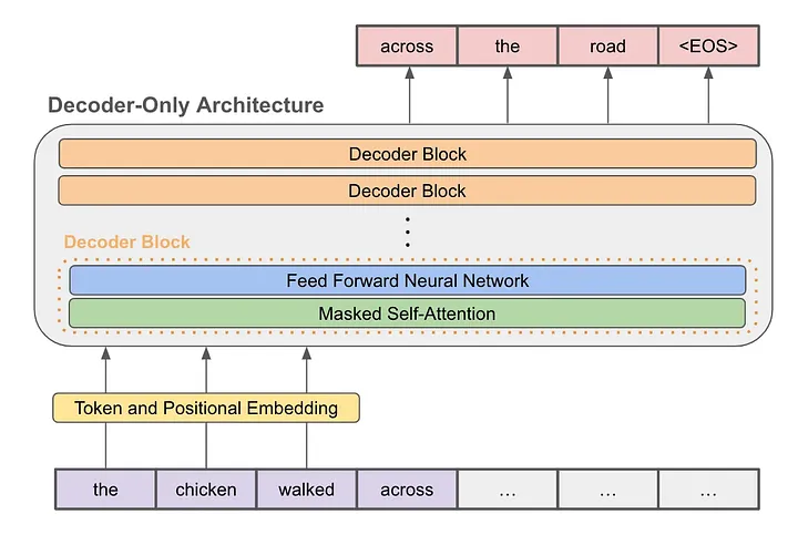
It is usually used for GPT-style tasks such as text generation and dialogue generation. The masking mechanism ensures that the decoder can only see the sequence already generated and cannot see future sequence elements.

The figure below shows the structure of a typical Decoder-Only model:

7. The Role of the Feed-Forward Network Layer

Qwen2MLP serves as the feed-forward network layer within the encoder or decoder module of the Transformer architecture; its role is to further apply nonlinear transformation and information integration to the features after the multi-head self-attention mechanism has processed the sequence information.

The feed-forward network layer usually consists of the following two main steps:

1. Linear transformation, which weights the input

It can be expressed by the formula y=Wx+b, where W is the weight matrix, b is the bias vector, x is the input vector, and y is the output vector.

2. A nonlinear activation function, which increases the model’s expressiveness

It can be expressed by the formula y=f(Wx+b), where f is the activation function, used to control the degree of neuron activation.

Common activation functions include ReLU, GELU, SiLU, and others.

During training, the feed-forward network layer needs to continuously adjust the weight matrix W and the bias vector b so that the model can better fit the training data.

8. The Role of RMSNorm Normalization

There are two questions:

1. Why normalize

Normalization removes scale differences in the input and reduces the input’s range of variation, which helps the model converge more easily during training

2. Why use RMSNorm

RMSNorm is a new normalization method based on the root mean square. Compared with traditional normalization methods such as BatchNorm and LayerNorm, its main advantage is that it does not need to compute the mean of the sample, giving a 40% speed improvement.

9. RoPE Rotary Position Embedding

A pure Attention module cannot capture the order of the input, that is, it cannot understand that tokens at different positions carry different meanings.

The core idea of RoPE is to multiply the positional encoding with the word vector via a rotation matrix, so that the word vector not only contains the semantic information of the vocabulary but also incorporates positional information. It has the following advantages:

1. Relative position awareness: RoPE can naturally capture the relative positional relationships between vocabulary items.
2. No extra computation: combining the positional encoding with the word vector is computationally efficient.
3. Adapts to sequences of different lengths: RoPE can flexibly handle input sequences of varying lengths.