1. What Is Bloom Filter

A Bloom Filter is a data structure proposed by Bloom in 1970.
It maps elements (x, y, z) through a series of functions into a binary vector (a 0101 sequence), and is used to quickly determine whether an element w is in a set. As shown below (from Wikipedia):

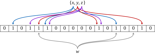
Compared with using a single mapping function, multiple mapping functions reduce the collision rate within the same address space. Therefore, at the same collision rate, multiple mapping functions require less address space than a single one.

A Bloom Filter uses a very short binary vector and achieves extremely high space efficiency by sacrificing accuracy. In large-scale data query scenarios, it effectively avoids disk IO and delivers very high query efficiency.

In fact, to determine whether an element is in a large set, you can also use a Bitmap. Convert the element to an integer x; the index value of x in the Bitmap is 0 (meaning it does not exist) or 1 (meaning it exists).

A Bloom Filter and a Bitmap are somewhat similar; both use a binary vector and mapping functions to determine whether an element exists. The difference is that a Bitmap has only one mapping function and its vector size cannot be smaller than the largest integer; a Bloom Filter has multiple mapping functions and can choose binary vectors of different sizes according to the false positive rate required by the scenario.

2. Common Application Scenarios

A Bloom Filter has a certain false positive rate and mainly solves two kinds of problems: definitely not present and possibly present.

2.1 Definitely Not Present - False

• Word spell checking. A misspelled word definitely does not exist
• Preventing database penetration. Querying rows or columns that do not exist
• Cache penetration. When nothing is found in the cache, the request penetrates to the database

2.2 Possibly Present - True

• Deduplicating URLs in a crawler. Skipping URLs that have already been crawled
• Spam filtering. Addresses on the blacklist are blocked
• Avoiding recommending duplicate articles. Skipping the URL/ID of articles already read
• Web interceptors. Blocking URL addresses on the blacklist

3. Choosing Bloom Filter Parameters

As mentioned above, a Bloom Filter can choose binary vectors of different sizes according to the false positive rate required by the scenario. In production we need to balance the false positive rate against efficiency. The formula given by Wikipedia is:

k = (m/n) ln2

where,

• m is the size of the binary vector
• n is the number of elements
• k is the number of mapping functions
• ln2 is a constant, approximately 0.69

The table below shows the false positive rate for different m/n and k.

When using it, first decide on an acceptable false positive rate, then compute the size of the binary vector from the formula:

m = (k * n) / ln2

For example, choose a false positive rate of 0.003, k = 4, m/n = 15 . With 1 million records, the required binary vector size is ( 4 _ 10e6 ) / 0.693 ≈ 5.77 _ 10e6 bit = 704.6 KB .

4. Drawbacks of Bloom Filter

The main drawbacks of a Bloom Filter:

1. Elements cannot be deleted. A single binary vector bit may correspond to the mappings of multiple elements, so it cannot simply be set to 0 .
2. It applies only to single-machine systems, and memory overhead grows linearly with data scale. Some middleware already provides Bloom filters, such as Redis, which can be used for very large-scale data scenarios.

There are many algorithms that optimize on the Bloom Filter; they amount to adding redundancy to the information, but none match the Bloom Filter in efficiency. Here are a few related algorithms:

• Counting Bloom Filter

On top of the standard Bloom filter, each Bit is replaced by a counter; adding an element increments the count, and deleting an element decrements it.

• Spectral Bloom Filters

In the Counting Bloom Filter above, the counters have a fixed number of bits. Spectral Bloom Filters use dynamically sized counters, which is more flexible and avoids counter overflow.

• Compressed Bloom Filters

By reducing the number of mapping functions, it reduces the Bits transmitted over the network. In exchange for the same false positive rate, the binary vector becomes larger.

• D-left Counting Bloom Filters

Based on D-left Hashing, it reduces storage space and the false positive rate, and supports element deletion.

• Dynamic Counting Filters

Supports querying the storage frequency of an element

• Cuckoo Filter

The cuckoo algorithm differs from the Bloom filter; it imitates the cuckoo to resolve mapping collisions. When different elements map to the same bit, the last mapped element kicks out the previously mapped one.

The cuckoo algorithm supports deletion, has a space utilization of only 50 %, stores only the fingerprint of an element, and has very high query efficiency.

5. Go Implementation

Here we use github.com/willf/bloom to run a simple test of the Bloom Filter.

 1
 2
 3
 4
 5
 6
 7
 8
 9
10
11
12
13
14
15
16
17
18
19

package main

import (
	"fmt"
	"github.com/willf/bloom"
)

func main() {
	n := uint(10000)
	error_rate := 0.003
	need_m, need_k := bloom.EstimateParameters(n, error_rate)
	fmt.Printf("Set m = %d , k = %d \n", need_m, need_k)
	filter := bloom.New(need_m, need_k)
	for i := 0; i < int(n); i++ {
		filter.Add([]byte(fmt.Sprintf("https://www.chenshaowen.com/%d", i)))
	}
	fmt.Println(filter.Test([]byte(fmt.Sprintf("https://www.chenshaowen.com/%d", 10000))))
	fmt.Printf("Done")
}

Execution result:

1
2
3

Set m = 120910 , k = 9
false
Done

6. References

• http://pages.cs.wisc.edu/~cao/papers/summary-cache/node8.html
• https://en.wikipedia.org/wiki/Bloom_filter
• https://github.com/willf/bloom