Interactive Notebook - Jupyter – Shaowen Chen's Website

1. Introduction

Jupyter Notebook (formerly IPython notebook) is an interactive notebook that supports running more than 40 programming languages.

Jupyter Notebook is in fact a web application that lets you create and share program documents, with support for live code, mathematical equations, visualizations, and Markdown. Its uses include data cleaning and transformation, numerical simulation, statistical modeling, machine learning, and more.

2. Local Installation

2.1 Local Installation

Anaconda is recommended, as it ships with Numpy, Scipy, Matplotlib, and many other Python development packages plus Jupyter notebook.

If you use a standalone Python interpreter, you need to install Jupyter:

1
pip install jupyter

2.2 Running Locally

1
jupyter notebook

3. Installing Jupyter with Docker

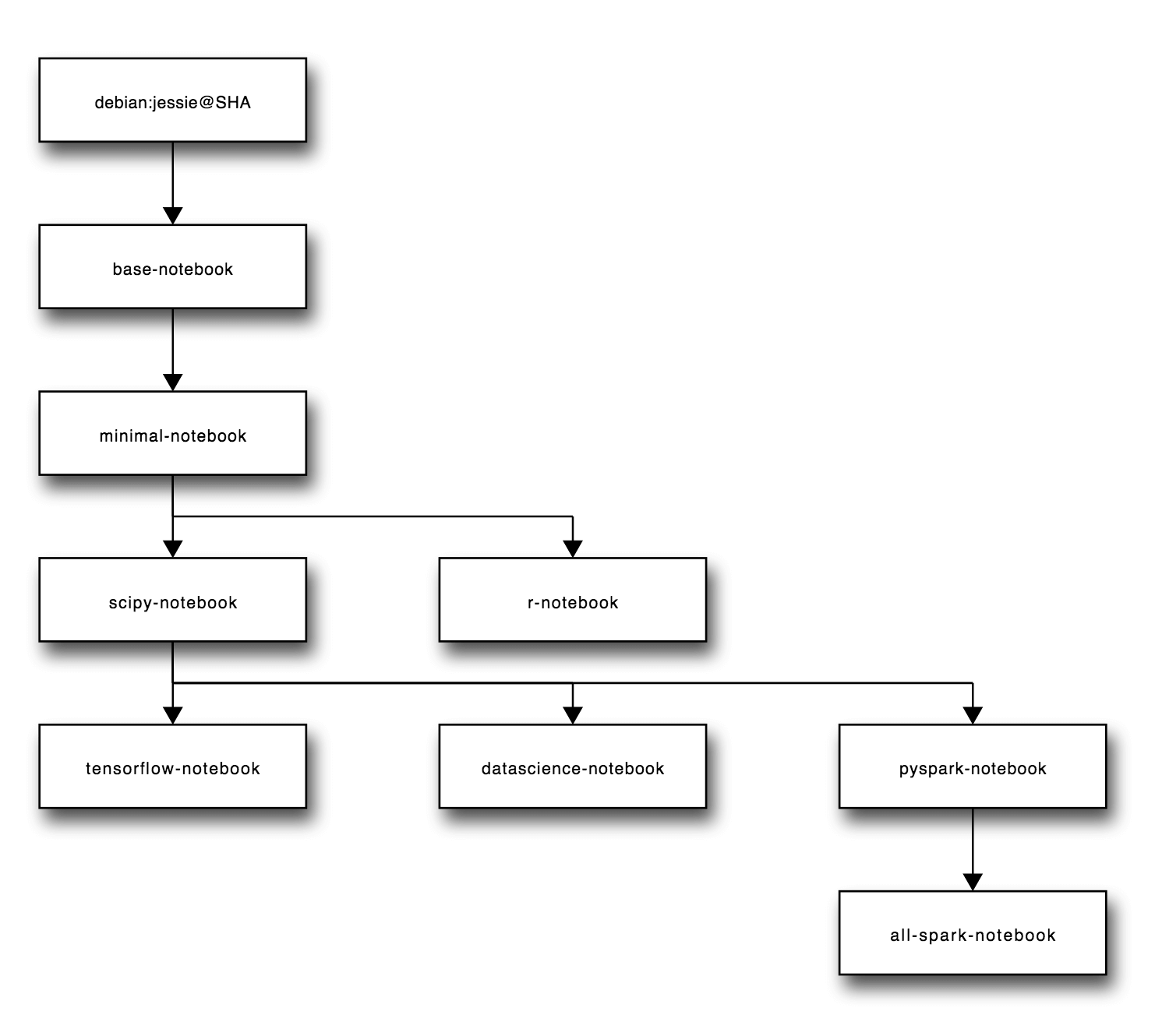
The official project offers base-notebook, minimal-notebook, all-spark-notebook, pyspark-notebook, scipy-notebook, datascience-notebook, tensorflow-notebook, and r-notebook. Pick the image that fits your needs.

3.1 Installing Docker

1
2
3
4
# CentOS 7 上安装 Docker
yum install docker
# 启动 docker 服务进程
service docker start

3.2 Running Jupyter

 1
 2
 3
 4
 5
 6
 7
 8
 9
10
11
docker run -d --security-opt apparmor=unconfined --security-opt seccomp=unconfined --name jupyter \
-p 8888:8888 \
--user root \
-e GRANT_SUDO=yes \
-e NB_UID=1000 \
-e NB_GID=100 \
-v /home/jupyter:/home/jovyan/work \
jupyter/tensorflow-notebook start-notebook.sh \
--NotebookApp.password='sha1:080ffe3b42b2:f592d77b83d318bad8ee771ba44a51569af552d8'
# 增加 NB_UID 对目录的权限
chown 1000 /home/jupyter

Parameter reference:

\ means a line continuation, splitting one command across multiple lines for readability
-d runs the started container in the background;
-p specifies the port; here the host’s port 8888 is mapped to the container’s port 8888;
–user=root allows running sudo;
-e specifies the permission-related IDs for the jovyan user;
–name sets a name for the started container;
-v mounts a host directory into the container. The Jupyter Docker document directory is /home/jovyan/work; so that documents survive the container being destroyed, the local directory /home/local/jupyter is mounted to /home/jovyan/work;
-NotebookApp.password is the login password, which you can generate in IPython with the following commands:

1
2
3
4
5
In [1]: from notebook.auth import passwd
In [2]: passwd()
Enter password: 123456
Verify password: 123456
Out[2]: 'sha1:080ffe3b42b2:f592d77b83d318bad8ee771ba44a51569af552d8'

3.3 Configuring Nginx

Use the nginx -t command to find the path of the Nginx configuration file. In nginx.conf, add the following:

 1
 2
 3
 4
 5
 6
 7
 8
 9
10
11
12
13
14
15
16
17
18
19
20
21
22
23
24
25
26
27
28
29
30
    upstream notebook {
        server localhost:8888;
    }
    server{
        listen 80;
        server_name yourdomain.com;
    location / {
        proxy_pass            http://notebook;
        proxy_set_header      Host $host;
        }

    location ~ /api/kernels/ {
        proxy_pass            http://notebook;
        proxy_set_header      Host $host;
        # websocket support
        proxy_http_version    1.1;
        proxy_set_header      Upgrade "websocket";
        proxy_set_header      Connection "Upgrade";
        proxy_read_timeout    86400;
        }
    location ~ /terminals/ {
        proxy_pass            http://notebook;
        proxy_set_header      Host $host;
        # websocket support
        proxy_http_version    1.1;
        proxy_set_header      Upgrade "websocket";
        proxy_set_header      Connection "Upgrade";
        proxy_read_timeout    86400;
        }
    }

Use nginx -s reload to restart the Nginx service and make it take effect.

4. Usage

Jupyter’s basic unit is a programming cell, that is, an In[ ]:

Jupyter has three types of cells: code, markdown cells, and raw cells, of which code cells and markdown cells are the ones commonly used.

Cells have two states, command mode and edit mode. Enter enters edit mode, ESC enters command mode, and both modes support many keyboard shortcuts.

Common command-mode shortcuts:

1
2
3
4
5
6
7
8
- y: 单元进入代码状态
- m: 转入markdown状态
- r：转入raw状态
- a: 上方插入新单元
- b：下方插入新单元
- x：剪切选中单元
- c: 复制选中单元
- shift-v：粘贴到上方单元

Inserting Markdown

Enter Markdown directly, then Run to render the result. Headings, text, videos, images and more are supported.

Inserting LaTeX formulas

Creating an inline formula

1
$\Gamma(n) = (n-1)!\quad\forall n\in\mathbb N$。

Block-level formula

1
$x = \dfrac{-b \pm \sqrt{b^2 - 4ac}}{2a} $$

Code blocks

You can output a code block directly on the page; just wrap it with ``` before and after ```.

Embedding images

1
2
from IPython.display import Image
Image(filename="yourpath.jpg")

Embedding music

You can embed both local music and music from the web

1
2
from IPython.display import Audio
Audio(filename="yourpath.wma")

1
2
from IPython.display import Audio
Audio(url="http://yourpath.wma")

Embedding a local video

 1
 2
 3
 4
 5
 6
 7
 8
 9
10
import io
import base64
from IPython.display import HTML

video = io.open('/home/test.mp4', 'r+b').read()
encoded = base64.b64encode(video)

HTML(data='''<video alt="test" controls>
     <source src="data:video/mp4;base64,{0}" type="video/mp4" />
     </video>'''.format(encoded.decode('ascii')))

Embedding a web page

1
2
from IPython.display import IFrame
IFrame('http://yourpath.com', width='100%', height=350)

Embedding a link

1
2
from IPython.display import FileLink
FileLink('./test/a.ipynb')

Magic commands

Every method starting with % is what is called a magic function, i.e. a method built into IPython. Note that magic methods come in two forms, % and %%, such as %timeit and %% timeit. IPython has specific names for them: the former is called line magic and the latter cell magic. As the names suggest, the former targets a single line of command while the latter targets multiple lines.

You can view all magic commands with %lsmagic, and use ? or ?? to view information about a command — the latter lets you see the source code. For example, %alias? brings up a description of that method.