1. Fractal Theory
1.1 The Definition of a Fractal
A fractal usually refers to a geometric shape that can be divided into several parts, each of which is approximately a reduced-scale copy of the whole — that is, it has the property of self-similarity.
1.2 The History of Fractal Research
In the 17th century, Leibniz already pondered the problem of self-similarity. In the 18th century, the study of continuous but non-differentiable functions by Karl Weierstrass, Georg Cantor, and Felix Hausdorff brought rigorous mathematical treatment to fractals.
The modern fractal craze, however, is inseparable from Mandelbrot. In 1967, the French-American mathematician Benoit Mandelbrot noticed that if kilometers are used as the unit of measurement, some of the winding stretches ranging from a few meters to a few dozen meters are ignored; switching to meters as the unit increases the measured total length, yet winding stretches below the centimeter scale still cannot be reflected; going further, theoretically, the next scale of seaside sand and gravel is molecules and atoms, so using ever smaller units of scale would yield a very different total length of coastline. Therefore, length is not a scale-independent invariant of a coastline. Mandelbrot introduced the new concept of “fractional-dimensional figures” and established the theory of fractal geometry that is well known today.
Starting in 1975, he successively published the works Fractals: Form, Chance and Dimension and The Fractal Geometry of Nature. Mandelbrot’s books received nothing like the attention they deserved from academia; only after 1982 did they draw widespread interest in European and American society, and they were later regarded by the fractal community as the “bible of fractal studies.”
1.3 Comparing Euclidean Geometry with Fractal Geometry
| Euclidean Geometry | Fractal Geometry |
|---|---|
| Classical (over 2000 years of history) | Modern mathematical monsters (over 30 years of history) |
| Based on characteristic length and proportion | No characteristic length or proportion |
| Suited to man-made artifacts | Suited to natural phenomena |
| Described by formulas | Described by (recursive or iterative) algorithms |
| Regular figures | Irregular figures |
| A finite number of structural levels in a figure | An infinite number of structural levels in a figure |
| A part generally does not carry the whole’s information | A part often carries the whole’s information |
| The more complex the figure, the more complex the rules behind it | The figure is complex, but the rules behind it are often simple |
2. Understanding Fractals
2.1 The Measurement Dimension of a Fractal
For an object of dimension d: when the unit of measurement changes to the original \(\frac{1}{r}\), the number of objects increases to \(r^d\). Expressed in logarithms, where d is the dimension, r is the magnification factor of the measurement, and k is the magnification factor of volume, then
$$d=log k/log r$$
Examples:
- After magnifying a line segment by two, the resulting segment can be seen as being formed by stacking 2 of the original segments.
- After magnifying a square by two, the resulting square can be seen as being formed by stacking \(2^2\) of the original squares.
- After magnifying a cube by two, the resulting cube can be seen as being formed by stacking \(2^3\) of the original cubes.
2.2 Julia Sets and Mandelbrot Sets
Consider the iteration of a complex function $$Z_{n+1} = {Z_n}^2+c, n=0,1,2……(1) $$
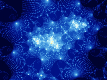
Fixing the complex parameter c, the distribution pattern in the complex plane of the initial values \(Z_0\) that make the iteration sequence {\(Z_n\)} bounded is called the Julia set, i.e. \(J_c=\) { \(Z_0|iteration sequence \){\(Z_n\)}\(is bounded \) }
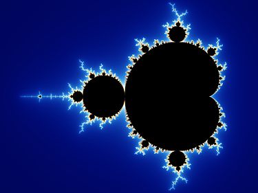
Fixing the initial value \(Z_0\), the distribution pattern in the complex plane of the parameters c that make the iteration sequence (1) bounded is called the Mandelbrot set. That is, \(J_c=\) { \(c|iteration sequence \){\(Z_n\)}\(is bounded \) }. Let $$Z=x+iy, c=p+iq$$
Then (1) becomes
$$
{
x_{n+1}={x_n}^2-{y_n}^2+p \\
y_{n+1}=2x_ny_n+q
}
$$
How to draw a Julia set:
- Set the initial values p,q, the maximum number of iterations N, the size of the figure a,b, and the number of colors K used. Note here that the modulus of c is always less than 2. It can be proven that when the modulus of c is greater than 2, the iteration will necessarily diverge to infinity.
- Set the boundary value of the region \( M\ge max(2,\sqrt{p^2+q^2}) \)
- Divide the region \(R=[-M,M]\times[-M,M]\) into an \(a\times b\) grid, and use each grid point as the initial value (\(x_0,y_0\)). Perform the iteration using the formula after the substitution above. If for all \(n \le N\) we have \({x_n}^2+{y_n}^2\le M^2 \), then set the pixel \((i, j)\) to this color. If starting from some step n we have \({x_n}^2+{y_n}^2\ge M^2 \), then set the pixel \((i, j)\) to a different color.
There is also an interesting theorem: a Julia set is either completely connected, with a path between any two points, or it is completely disconnected, with the entire figure consisting of isolated points.
How to draw a Mandelbrot set:
The algorithm is exactly the same as for Julia, except that here the x,y values are fixed as the initial values, while c is treated as the variable. Every point inside the Mandelbrot set corresponds to a connected Julia set, while points outside the Mandelbrot set correspond to disconnected Julia sets; the Mandelbrot figure is a thumbnail of the Julia sets.
One can therefore imagine that we have four variables x,y,p,q, and fixing any two of them while treating the other two as variables yields a different figure. If all the Julia sets were gathered together, one would obtain a four-dimensional figure.
