1. Koch Curve

The Swedish mathematician Helge von Koch proposed the Koch curve in his 1904 paper “On a continuous curve without tangents, constructible from elementary geometry.” It is described as follows:

1. Specify the length of a line segment \(l\) (this can be thought of as iteration 0)
2. Divide this segment into three equal parts, construct an equilateral triangle with the middle segment as its base, then remove the base
3. Repeat step 2 for every edge of the curve generated in step 2 (each operation is called one iteration)

The length of the resulting set figure is: $$L=l*(\frac{4}{3})^{N}$$, where N is the number of iterations.

1.2 Drawing method:

1. If N=0, just draw a straight line of length L
2. If N=1 (the first iteration), draw a segment of length L/3; turn the pen left 60 degrees and draw a segment of length L/3; turn the pen right 120 degrees and draw a segment of length L/3; then turn the pen left 60 degrees and draw a segment of length L/3

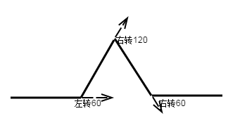
3. If n>1, the n-th iteration is equivalent to: n-1 iterations; turn the pen left 60 degrees; n-1 iterations; turn the pen right 120 degrees; n-1 iterations; turn the pen left 60 degrees; n-1 iterations.

1.3 Python code implementation

 1
 2
 3
 4
 5
 6
 7
 8
 9
10
11
12
13
14
15
16
17
18
19
20
21
22
23

# -*- coding: utf-8 -*-
import turtle

Division = 3.0
DirectionAangle = [('left',60),('right',120),('left',60)]

def call(name):
    if name == 'left':
        return turtle.left
    else:
        return turtle.right

def koch(n, length):
    if n==0:
        turtle.forward(length)
    else:
        for DA in DirectionAangle:
            koch(n-1,length/Division)
            call(DA[0])(DA[1])
        koch(n-1,length/Division)

koch(n=2, length=100)
turtle.done()

1.4 The figures drawn

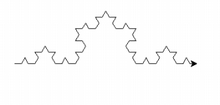
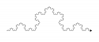
Below are the Koch curves generated with n=3, length=300 and n=4, length=400 respectively

2. Julia Set

2.1 Drawing method

As mentioned in the previous post, click here to go

1. Set the initial values p, q, the maximum number of iterations N, the figure size a, b, and the number of colors used K. Note here that the modulus of c is always less than 2. It can be proved that when the modulus of c is greater than 2, the iteration will necessarily diverge to infinity.
2. Set the boundary value of the region \( M\ge max(2,\sqrt{p^2+q^2}) \)
3. Divide the region \(R=[-M,M]\times[-M,M]\) into an \(a\times b\) grid, and use each grid point as the initial value (\(x_0,y_0\)). Iterate using the formula after the substitution above. If \({x_n}^2+{y_n}^2\le M^2 \) holds for all \(n \le N\), set pixel \((i, j)\) to this color. If from some step n onward \({x_n}^2+{y_n}^2\ge M^2 \), set pixel \((i, j)\) to a different color.

2.2 Python code implementation

 1
 2
 3
 4
 5
 6
 7
 8
 9
10
11
12
13
14
15
16
17
18
19
20
21
22
23
24
25
26
27
28
29
30

# -*- coding: utf-8 -*-

import matplotlib.pyplot as plot
import numpy as np
p=0.45 #初始值c的实部
q=-0.1428 #初始值c的虚部
N=800 #最大迭代次数
M=100 #迭代区域的界值
a=3.0 #绘制图的横轴大小
b=3.0 #绘制图的纵轴大小
step=0.005 #绘制点的步长

def iterate(z,N,M):
    z=z*z+c
    for i in xrange(N):
        if abs(z)>M:
            return i
        z=z*z+c
    return N

c=p+q*1j
i=np.arange(-a/2.0,a/2.0,step)
j=np.arange(b/2.0,-b/2.0,-step)
I,J=np.meshgrid(i, j)
ufunc=np.frompyfunc(iterate,3,1)
Z=ufunc(I+1j*J,N,M).astype(np.float)
plot.imshow(Z,extent=(-a/2.0,a/2.0,-b/2,b/2.0))
cb = plot.colorbar(orientation='vertical',shrink=1)
cb.set_label('iteration counts')
plot.show()

2.3 The figures drawn

Parameters: p=0.285 q=0.01 N=200 M=100 a=2.0 b=2.0 step=0.005 (left figure)

Parameters: p=0.45 q=-0.1428 N=200 M=100 a=2.0 b=2.0 step=0.005 (right figure)

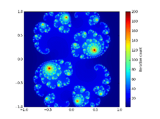
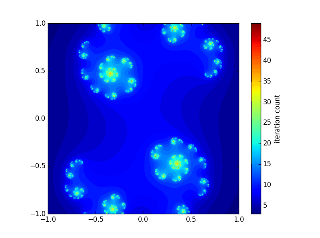
There are also other initial values of c that produce very beautiful patterns, for example:

c = -0.70176+-0.3842j
c = -0.835+-0.2321j
c = -0.8+0.156j
c = 0.285

3. Mandelbrot Set

Mathematical definition:
$$f_c(z) = z^2+c$$

The Mandelbrot set is the set of sequences for which the iteration of the function \(f_c(z)\), at z=0 with respect to the complex number c=x+yi, does not diverge.

The simplest way to draw the Mandelbrot set is to use escape time. Escape time refers to the number of iterations performed, within a specified range M and up to a finite count N, before the value leaves the region M. Different numbers of iterations are drawn in different colors.

1. Set the maximum number of iterations, N
2. Set the initial value of \(z_0\)
3. Set the escape radius R, usually 2

3.1 Drawing method

3.2 Python implementation

 1
 2
 3
 4
 5
 6
 7
 8
 9
10
11
12
13
14
15
16
17
18
19
20
21
22
23
24
25
26
27
28
29
30
31
32

# -*- coding: utf-8 -*-

import numpy as np
import matplotlib.pyplot as plot

x0=0 #初始值z0的x0
y0=0 #初始值z0的y0
zoom=1.0 #放大倍率
N=100 #最大迭代次数
R=2 #迭代半径
a=4.0 #绘制图的横轴大小
b=3.0 #绘制图的纵轴大小
step=0.005 #绘制点的步长

def iterate(c,N,R):
    z=c
    for i in xrange(N):
        if abs(z)>R:
            return i
        z = z*z+c
    return N

x=np.arange(-a/(2.0*zoom)+x0,a/(2.0*zoom)+x0,step)
y=np.arange(b/(2.0*zoom)+y0,-b/(2.0*zoom)+y0,-step)
cx,cy=np.meshgrid(x, y)
c = cx + cy*1j
ufunc=np.frompyfunc(iterate,3,1)
Z=ufunc(c,N,R).astype(np.float)
plot.imshow(Z,extent=(-a/2.0,a/2.0,-b/2,b/2.0))
cb = plot.colorbar(orientation='vertical',shrink=1)
cb.set_label('iteration counts')
plot.show()

3.3 The figures drawn

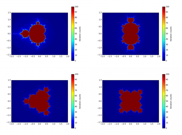
The figure shows the image generated using the parameters: x0=0 y0=0 zoom=1.0 N=100 R=2 a=4.0 b=3.0 step=0.005. The difference is that they use quadratic and cubic power iterations respectively.

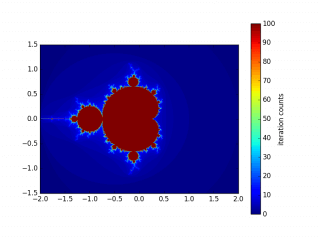
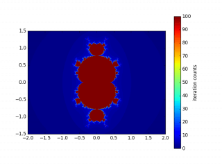
Finally, you can also use the ImageMagick tool to turn the generated images into an animated GIF.

1

convert *.png  out.gif